Experimental observation of the Hund's metal to bad metal crossover

A definitive experimental signature of the crossover from a Fermi liquid metal to a bad metal is the disappearance of a Drude peak in the optical conductivity. In single band systems this occurs in proximity to a Mott insulator and is particularly clearly seen in organic charge transfer salts and is nicely captured by Dynamical Mean-Field Theory (DMFT).

An important question concerning multi-band systems with Hund's rule coupling, such as iron-based superconductors, is whether there is a similar collapse of the Drude peak. This is clearly seen in one material in a recent paper

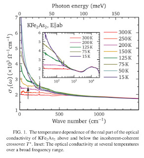
Observation of an emergent coherent state in the iron-based superconductor KFe2As2 
Run Yang, Zhiping Yin, Yilin Wang, Yaomin Dai, Hu Miao, Bing Xu, Xianggang Qiu, and Christopher C. Homes

Note how as the temperature increases from 15 K to 200 K that the Drude peak collapses. 

The authors give a detailed analysis of the shifts in spectral weight with varying temperature by fitting the optical conductivity (and reflectivity from which it is derived) at each temperature to a model consisting of three Drude peaks and two Lorentzian peaks. Note this involves twelve parameters and so one should always worry about the elephants trunk wiggling.

On the other hand, they do the fit without the third peak, which is of the greatest interest as it is the sharpest and most temperature dependent, and claim it cannot describe the data.

The authors also perform DFT+DMFT calculations of the one-electron spectral function (but not the optical conductivity) and find it does give a coherent-incoherent crossover consistent with the experiment. However, the variation in quasi-particle weight with temperature is relatively small.

Conducting metallic-organic frameworks

Thanks to the ingenuity of synthetic chemists metallic-organic frameworks (MOFs) represent a fascinating class of materials with many potential technological applications.
Previously, I have posted about spin-crossover, self-diffusion of small hydrocarbons, and the lack of reproducibility of CO2 absorption measurements in these materials.

At the last condensed matter theory group meeting we had an open discussion about this JACS paper.
Metallic Conductivity in a Two-Dimensional Cobalt Dithiolene Metal−Organic Framework 
Andrew J. Clough, Jonathan M. Skelton, Courtney A. Downes, Ashley A. de la Rosa, Joseph W. Yoo, Aron Walsh, Brent C. Melot, and Smaranda C. Marinescu

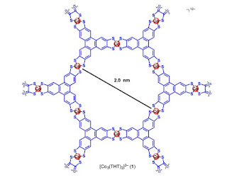
The basic molecular unit is shown below. These molecules stack on top of one another, producing a layered crystal structure. DFT calculations suggest that the largest molecular overlap (and conductivity) is in the stacking direction.
Within the layers the MOF has the structure of a honeycomb lattice.

The authors measured the resistivity of several different samples as a function of temperature. The results are shown below. The distances correspond to the size of the compressed powder pellets.

Based on the observation that the resistivity is a non-monotonic function of temperature they suggest that as the temperature decreases there is a transition from an insulator to a metal. Since there is no hysteresis they rule out a first-order phase transition, as is observed in vanadium oxide, VO2.
They claim that the material is an insulator about about 150 K, based on fitting the resistivity versus temperature to an activated form, deducing an energy gap of about 100 meV. However, one should note the following.

1. It is very difficult to accurately measure the resistivity of materials, particularly anisotropic ones. Some people spend their whole career focussing on doing this well.

2. Measurements on powder pellets will contain a mixture of the effects of the crystal anisotropy, random grain directions, intergrain conductivity, and contact resistances. This is reflected in how sample dependent the results are above.

3. The measured resistivity is orders of magnitude larger than the Mott-Ioffe-Regel limit. suggesting the samples are very "dirty" or one is not measuring the intrinsic conductivity or this is a very bad metal due to electron correlations.

4. It is debatable whether one can deduce activated behaviour from only an order of magnitude variation in resistance, due to the narrow temperature range considered.

The temperature dependence of the magnetic susceptibility is shown below, and taken from the Supplementary material.

The authors fit this to a sum of several terms, including a constant term and a Curie-Weiss term. The latter gives a magnetic moment associated with S=1/2, as expected for the cobalt ions, and an antiferromagnetic exchange interaction J ~ 100 K. This is what you expect if the system is a Mott insulator or a very bad metal, close to a Mott transition.

Again, there a few questions one should be concerned about.

1. How does this relate to the claim of a metal at low temperatures?

2. The problem of curve fitting. Can one really separate out the different contributions?

3. Are the low moments due to magnetic impurities?

The published DFT-based calculations suggest the material should be a metal because the bands are partially full. Electron correlations could change that. The band structure is quasi-one-dimensional with the most conducting direction perpendicular to the plane of the molecules.

All these questions highlight to me the problem of multi-disciplinary papers. Should you believe physical measurements published by chemists? Should you believe chemical compositions claimed by physicists? Should you believe theoretical calculations performed by experimentalists? We need each other and due diligence, caution, and cross-checking.

Having these discussions in group meetings is important, particularly for students to see they should not automatically believe what they read in "high impact" journals?

An important next step is to come up with a well-justified effective lattice Hamiltonian.

Desperately seeking organic spin liquids

A spin liquid is a state of matter where there is no magnetic order (spontaneous breaking of spin rotational symmetry) at zero temperature. The past few decades has seen a desperate search for both real materials and Heisenberg spin models in two spatial dimensions that have this property. I have written many posts on the subject. An important question is what is a definitive experimental signature of such a system.

Strong candidate materials are the Mott insulating phase of several organic charge transfer salts, which was reviewed in detail in 2011 by Ben Powell and I.

One experimental signature is the temperature dependence of the specific heat. In particular, some theories predict spin liquid states with spinon excitations with a Fermi surface. This would lead to a linear term in the temperature dependence of the specific heat, as one sees in a simple metal that is a Landau Fermi liquid. This paper is one of several that claims to observe this signature.

However, it is important to bear in mind two subtle issues with interpreting these experiments. 

First, one always have to subtract off the large contribution to the specific heat from lattice vibrations. There are two main ways to do this. One is to fit the data, including a cubic term, T^3 in the temperature dependence. The second method is to subtract the data from a different compound (e.g. a deuterated one) which has a different electronic (magnetic) ground state but a similar crystal structure. Due to subtle isotope effects and hydrogen bonding, sometimes deuterated compounds are argued to meet this requirement for the magnetic contributions to be different and the phonon contributions to be the same.

However, there are problems with both of these subtraction methods. 

First, curve fitting with many parameters can be getting the tail of the elephant to wiggle, as discussed more below. Second, changing the chemistry does change the phonon spectrum and so also changes the lattice contribution.

Finally, what about the linear in T term? 

In a News and Views about a 2008 Nature Physics paper claiming to observe this linear in T term, Art Ramirez showed one could take the same experimental data and fit it to an alternative expression involving T^(2/3) which was proposed by an alternative theory. 

This is shown in the Figure below.

I also worry about how the low T specific heat is dominated by the 1/T^2 term associated with the Schottky anomaly from two level systems.

Unfortunately, Ramirez's concerns seem to have been ignored in following papers.

We really need more direct experimental probes of spin liquid behaviour. Unfortunately, there is a paucity of realistic ones.

A basic but important skill: critical reading of experimental papers

Previously, I highlighted the important but basic skill of being skeptical. Here I expand on the idea.

An experimental paper may make a claim, "We have observed interesting/exciting/exotic effect C in material A by measuring B."
How do you critically assess such claims?
Here are three issues to consider.
It is as simple as ABC!

1. The material used in the experiment may not be pure A.
Preparing pure samples, particularly "single" crystals of a specific material of know chemical composition is an art. Any sample will be slightly inhomogeneous and will contain some chemical impurities, defects, ... Furthermore, samples are prone to oxidation, surface reconstruction, interaction with water, ... A protein may not be in the native state...
Even in a ultracold atom experiment one may have chemically pure A, but the actual density profile and temperature may not be what is thought.
There are all sorts of checks one can do to characterise the structure and chemical composition of  the sample. Some people are very careful. Others are not. But, even for the careful and reputable things can go wrong.

2. The output of the measurement device may not actually be a measurement of B.
For example, just because the ohm meter gives an electrical resistance does not mean that is the electrical resistance of the material in the desired current direction. There are all sorts of things that can go wrong with resistances in the electrical contacts and in the current path within the sample.
Again there are all sorts of consistency checks one can make. Some people are very careful. Others are not. But, even for the careful and reputable things can go wrong.

3. Deducing effect C from the data for B is rarely straightforward.
Often there is significant theory involved. Sometimes, there is a lot of curve fitting. Furthermore, one needs to consider alternative (often more mundane) explanations for the data.
 Again there are all sorts of consistency checks one can make. Some people are very careful. Others are not. But, even for the careful and reputable things can go wrong.

Finally, one should consider whether the results are consistent with earlier work. If not, why not?

Later, I will post about critical reading of theoretical papers.

Can you think of other considerations for critical reading of experimental papers?
I have tried to keep it simple here.

I believe in irreproducible results

At UQ we just had an interesting colloquium from Signe Riemer-Sorensen about Dark matter emission - seeing the invisible. Central to the talk was the data below. Focus on the red data around 3.6 keV.

This has stimulated more than 100 theory papers!
This reminds me of the faster than speed of light neutrinos and the 17 keV neutrino, 500 GeV particles seen by the Fermi gamma ray telescope, BICEP2 "evidence" for cosmic inflation, ....

The above data is discussed in detail here.

I don't want to just pick on my astrophysics and high energy physics colleagues as this happens in condensed matter and chemistry too... remember cold fusion... think about periodic reports of room temperature superconductors!

The painful reality is that cutting edge science is hard. One can be incredibly careful about noise, subtracting background signals, statistical analysis, sample preparation, .... but in the end there is Murphy's law .... things do go wrong .... and crap happens...

Skepticism and caution should always be the default reaction; all the more so the greater the possible significance or surprise of the "observed" result.

I believe in irreproducible results.

Update (14 December).
Clifford Taubes brought to my attention two relevant papers on the possible 3.5 keV line. The first paper rules out a dark matter origin of the line and even mentions Occam's razor. The second has a mundane alternative explanation of the line in terms of charge exchange between hydrogen gas and sulfur ions.

How robust are your tight-binding model parameters?

In a previous post I discussed the problem of extracting reliable parameters for tight-binding (and Hubbard) models from ab initio band structure calculations. My comments then were influenced by the figure below, which has now appeared on the arXiv in a short review by Anthony Jacko.

First, the band structure for a specific organic material was calculated using a density functional theory (DFT) based approximation. The energy dispersion relations were then fit to a tight-binding model involving 8 different hopping integrals, t0, t1, ....t7. 

The horizontal axis indexes the 8 integrals, the vertical axis shows their values determined from a range of different fits, using slightly different fitting methods and different runs of the fitting algorithm. 

Note the significant differences.
Thus, caution is in order if one uses the common practise of simply performing one fit [which may look impressive to the naked eye].
Jacko notes that this is like getting the elephants trunk to wiggle.

As Jacko stresses in the review, the most reliable and physically transparent way to determine the tight-binding hopping integrals is to construct Wannier orbitals and then directly calculate the integrals. The results for that procedure are shown in green. The red curve is the global best fit.

Cherry picking theories

Cherry picking data is not just done by scientific "denialists" but also some "respected" theorists who are seeking support for their scientific theory.

I recently realised that some experimentalists cherry pick theories to describe their experimental data. I heard a talk by a theorist who reported having several disturbing conversations along the following lines.

Experimentalist: We fitted our data to your theory.

Theorist: But the theory is not valid or relevant in the parameter regime of your experiment.

Experimentalist: We don't care. The theory fits the data.

Common challenges with constructing diabatic states and tight-binding models

I wish to highlight some common issues that occur in the construction, justification and parametrisation of effective Hamiltonians in both theoretical chemistry and solid state physics.
The basic issue is one needs to keep in mind that just because one gets the energy eigenvalues of a quantum system "correct" does not mean that one necessarily has the correct wave function.
Previously, I posted how sometimes a variational wave function can give  a good ground state energy but be qualitatively incorrect.

For molecular systems a powerful approach to understanding the potential energy surfaces of the ground state and the lowest lying electronic states is to construct a Hamiltonian matrix based on a few diabatic states.

For crystals in which the electronic degrees of freedom are strongly correlated a powerful approach is to construct a Hubbard model where the non-interacting band structure is described by a tight-binding model. The latter describes hopping of electrons between orbitals that are localised on individual lattice sites.

Quantum chemistry
There are two strategies that are used to construct and parametrise a diabatic state model.

1. Based on chemical insight one writes down a Hamiltonian of the form

One assumes some functional form for the Hamiltonian matrix elements, with several free parameters.
One calculates the adiabatic potential energy surfaces using an ab initio method and fits these surfaces to the adiabatic energies from the diabatic model.
An example is shown below for a two-state diabatic model for fluorescent protein chromophores.

The  example below concerns five electronic states of XH3 and the associated torsional potential, taken from this paper. There are 11 free parameters in the Hamiltonian.

A different approach by Nangia and Truhlar considers a multi-dimensional potential surface for ammonia, two diabatic states, and hundreds of free parameters.

Important questions arise.
Are the diabatic states physical?
Or is all this curve fitting just making the elephants trunk to wiggle? 
As one includes more diabatic states how does one deal with the confusion and ambiguity that arises because of the close proximity to one another of many excited states?

2. A more rigorous approach is to use some well-defined procedure to actually construct the diabatic states from a knowledge of the many-body wave functions of the low lying states. An example is the approach pioneered by Cederbaum. Seth Olsen has nicely used this approach to construct diabatic states for fluorescent protein chromophores and other organic dyes. Furthermore, the diabatic states can be related to chemically intuitive valence bond structures.
However, subtle issues still arise, particularly as one includes more excited states.

Solid state physics
Similarly, there are two strategies that are used to construct and parametrise a tight-binding model for a specific material.

1. One writes down a tight-binding model Hamiltonian with a few parameters describing hopping integrals and calculates the associated band structure. One then calculates the band structure for a specific material, using an ab initio method, usually some approximation of Density Functional Theory (DFT). One then fits this band structure to the tight-binding model in order to determine the hopping integrals.

An example is shown below, taken from this paper. The green dots are from an DFT based calculation and the solid black lines are a fit to a tight-binding model with a few free parameters.

This procedure gets messy and ambiguous when in order to improve the quality of the fit one starts to introduce extra parameters representing beyond next-nearest neighbour hopping. 

Are such long range hoppings justified? Furthermore, the parameter values obtained can vary significantly as one introduces extra parameters.

2. A more rigorous approach is to construct Wannier orbitals and then calculate the actual overlap integrals that are input into a tight-binding model.
An example is in this paper concerning the Fabre salts. In particular it shows how some longer range hoppings are actually justified.
However, there are many subtleties and ambiguities in this approach as discussed in a recent Reviews of Modern Physics. This tends to work well when there are a couple of well isolated bands, but not otherwise.

Clearly, 2. is always preferable because it has a stronger physical basis. However, it is not easy. People tend to be just do 1. with a fixed number of parameters and not worry about whether they are justified or stable.

I thank Seth Olsen and Anthony Jacko for teaching me about these issues.

Mapping quasi-particles in strongly interacting ultra cold fermionic gases

There is an interesting preprint
Breakdown of Fermi liquid description for strongly interacting fermions 
Yoav Sagi, Tara E. Drake, Rabin Paudel, Roman Chapurin, Deborah S. Jin

It describes some nice ultra cold atom experiments that tune through the BEC-BCS crossover with a Feshbach resonance, focusing on the properties of the normal (i.e. non-superfluid) phase. All the measurements are at a temperature of T=0.2T_F, just above the superfluid transition.
It is like an ARPES [Angle Resolved PhotoEmission Spectroscopy] experiment in the solid state.
Specifically, the one-fermion spectral function A(k,E) is measured, shown in the colour intensity plots below.

The left and right side correspond to the BCS and BEC limits respectively. The unitary limit [i.e. infinite interaction occurs close to the middle].

On the left one can clearly see dispersing quasi-particle excitations, as one would expect in a Fermi liquid. As the interaction strength increases this feature is broader and there is more incoherent spectral weight at lower energies.

Some caution is in order as there is quite a bit of curve fitting involved in the analysis of the above data. [Solid state ARPES also suffers from this problem to.]

Specifically, the form below is used for the spectral function, where Z is the quasi-particle weight

In an earlier post I considered the history of this type of expression.

For the incoherent part the authors make the somewhat ad hoc assumption that it is given by a
 "function that describes the normal state in the BEC limit, namely, a thermal gas of pairs."

They then find the following results for the dependence of Z and the effective mass m* [defined by the quadratic dispersion] on the interaction strength [a is the scattering length, which becomes infinite at the Feshbach resonance, i.e. for the unitary limit].

There is already a theory paper that discusses the experiments. It captures the results above at the semi-quantitative level using a Brueckner-Goldstone theory. The self energy is assumed to be frequency independent in this approximation. I found this interesting as it is the opposite to Dynamical Mean-Field Theory (DMFT) for which the self energy is assumed to be momentum independent.

I feel the paper title may be a misnomer. The quasi-particle weight is always finite, except in the BEC regime [attractive interactions] where one does not really have fermions anymore.

In future experiments, it would be nice to see the temperature dependence of the spectral function. Specifically, do the quasi-particles get destroyed with increasing temperature as in bad metals.

I thank Matt Davis for bringing the preprint to my attention.

Why am I skeptical about curve fitting?

It continues to amaze and frustrate me how some people will do the following.
Take experimental data for a specific quantity [e.g. resistivity vs. temperature].
Fit the data to a function from some exotic theory X involving N free parameters.
Claim that the "successful" fit "proves" that X is the correct theory.

Why am I skeptical? What would it take to convince me X is actually valid?

1. Have N < 4, remembering the elephants wiggling trunk.
2. With the same set of parameters also fit at least one, and preferably several,  other experimental observation [e.g. thermopower vs. temperature].
3. Show that the fit parameters are physically reasonable and consistent with estimates from independent determinations. Science is all about comparisons.
4. Also fit the data to the predictions of mundane theory M, and alternative exotic theory X2, and clearly show they cannot fit the data. i.e., apply the method of multiple alternative hypotheses.

Finally, there is a more profound philosophical point, the underdetermination of scientific theory. We can never be sure there are not alternative theories we have not considered.

When is curve fitting valid and useful? What does it take to convince you?

Water: anomalies, challenges, and controversies

I really enjoyed this week's meeting Water: the most anomalous liquid at NORDITA. This is the first time I have ever been to a workshop or conference that is solely about water. Here are some impressions and a few things I learnt as a newcomer to the field.

Just how unique and anomalous is water?
Not as unique as I thought. Some other tetrahedral liquids have similar properties.

Hydrogen bonding is not what makes water unique
Rather it is the tetrahedral character of the intermolecular interactions that arise from hydrogen bonding. This distinction can be seen from the fact that the mW (monatomic water) model captures many of the unusual properties of water.

DFT is a nightmare
I have written a number of posts that express caution/concern/alarm/skepticism about attempts to use Density functional theory (DFT) to describe properties of complex materials. Trying to use it to calculate properties of a liquid water in thermal equilibrium is particularly adventurous/ambitious/reckless. First, there is the basic question: can it even get the properties of a water dimer in the gas phase correct? But, even if you choose a functional and basis set so you get something reasonable for a dimer there is another level of complexity/fakery/danger associated with "converging" a molecular dynamics simulation with DFT producing the Born-Oppenheimer surface. This was highlighted by several speakers. Simulations need to give error bars!

A physically realistic force field (at last!)
A plethora of force fields [TIP3P, SPC/E, TIP4P/2005, ST2, ....] have been developed for classical molecular dynamic simulations. They are largely based on electrostatic considerations and involve many parameters. The latter are chosen in order to best fit a selection of experimental properties [melting temperature, temperature of maximum density, pair correlation function, dielectric constant, ....]. Some models use different force fields for ice and liquid water. On the positive side it is impressive how some of these models can capture qualitative features of the phase diagram including different ice phases and give a number of experimental properties within a factor of two. On the negative side: they involve many parameters, it is hard to justify including some "forces" and not others, and give very poor values for some experimental observables [e.g. TIP3P has ice melting at 146 K!]. How often do people get the right answer for the wrong reason?

An alternative strategy is to actually calculate an ab initio force field using state of the art quantum chemistry and a many-body expansion that includes not just two-body interactions (i.e. forces between pairs of molecules) but three-body and beyond interactions. This was discussed by Sotiris Xantheas and Francesco Paesani. An end result is MB-pol.

Quantum zero-point energy is (not) important
Sotiris Xantheas emphasised that semi-empirical force fields are effective Hamiltonians that implicitly include quantum nuclear effects at some effective classical potential [e.g. a la Feynman-Hibbs]. Thus, if one then does a path integral simulation using one of these force fields one is  "double counting" the quantum nuclear effects at some level. Xantheas and Paesani also emphasised that MB-pol should not be expected to agree with experiment unless nuclear quantum effects are included.
On the other hand, due to competing quantum effects classical simulations for water give better results than one might expect.

The elusive liquid-liquid critical point
Some of this controversy reminded me of high-Tc cuprate superconductors where the elusive quantum critical point [under the superconducting dome?] may (or may not) exist. It is also interesting that there is a proposal of a Widom line in the cuprates, perhaps inspired by water.
Some of the arguments and sociology seemed like the cuprates. There are true believers and non-believers. Each camp interprets (and criticises) complicated and ambiguous experimental results and large computer simulations according to their prior beliefs. Kauzmann's maxim is relevant: people will often believe what they want to believe rather than what the evidence before them suggests they should believe.

Perhaps this critical point does not appear in the physical phase diagram of bulk water but can be accessed via "negative pressure" in some force field models. A key observable to calculate is the heat capacity, experimentally it appears to diverge. But its calculation will require inclusion of nuclear quantum effects. [It is not clear to me why you can't just input the classical vibrational spectrum into a non-interacting quantum partition function.]

I felt this issue dominated some discussions at the meeting too much.

The O-O radial distribution function is over-emphasised
In any liquid this pair correlation function is an important observable that is a measure of the amount of structure in the liquid. For water the O-O radial function has been "accurately" measured and provides a benchmark for theories. Getting it correct is a necessary but not a sufficient condition for having a correct theory. But water is an anisotropic molecular liquid not a Lennard-Jones monatomic fluid. Angular correlations are very important for water. Also, unfortunately, other pair correlation functions such as the O-H and H-H radial distribution functions are not well characterised experimentally.

When are the many-body effects quantum?
One can make many-body expansions in electrostatics, classical statistical mechanics, and quantum many-body theory. A profound question is: are there situations, criteria, or properties that can make the latter distinctly different from the former?

How good should parameterisation of simple models be?

Over the past few years I have advocated a simple diabatic state model to describe hydrogen bonding in a diverse range of molecular complexes. In my first paper I suggested the following parameterisation of the matrix element coupling the two diabatic states

with two free parameters Delta1 and b, which describe the energy scale and length scale for the interaction.
R1 is just a reference distance ~ 2.4 A, introduced so that the prefactor Delta1 corresponds to a physically relevant scale.
The two parameter values I chose give a quantitative description of a wide range of properties [bond lengths, vibrational frequencies, and the associated isotope effects, when the quantum nuclear motion is taken into account.

Last week I found this nice paper
Solvent-Induced Red-Shifts for the Proton Stretch Vibrational Frequency in a Hydrogen-Bonded Complex. 1. A Valence Bond-Based Theoretical Approach 
Philip M. Kiefer, Ehud Pines, Dina Pines, and James T. Hynes

It uses a similar two-diabatic state model and references earlier work of Hynes going back to 1991. A parameterisation like that above is used.

Below is a plot of Delta (kcal/mol) vs. R (Angstroms), comparing my parametrisation to Hynes.

The curve with the smaller slope is the parameterisation of Hynes.

I found this agreement very satisfying and encouraging. I have mostly been concerned with symmetrical complexes [where the proton affinity of the donor and acceptor is equal] and bonds of strong to moderate strength [R ~ 2.3-2.6 Angstroms] and have compared the theory to experimental data for solid state materials. In contrast, Hynes has been mostly concerned with asymmetric complexes in polar solvents with weaker bonds [R ~ 2.7-2.8 Angstroms].

I also felt bad that I had not referenced Hynes work. Then I went back and checked my first paper. To my relief, I found I had explicitly stated that the parameterisation in his 1991 paper was comparable to mine. It is amazing how quickly I forget stuff!

But the main point of this post is to raise two general questions.

1. Should I really be so happy? Aren't I missing the point of simple models: to give insight into the essential physics and chemistry and describe trends in diverse set of systems. All that matters is that the parameters are "reasonable", i.e. not crazy.

2. What is a reasonable expectation for consistent parametrisation of simple models? At what point does one abandon a model because it requires some parameters that are "unreasonable"? For example, if Hynes parameters differed by a factor of ten or more I would say there is a serious problem with the model. But I would not be that concerned by a 50 per cent discrepancy.

Here is a concrete example for 2. At a recent Telluride meeting, Dominika Zgid lampooned the fact that for cerium oxides, people doing DFT+U calculations have used values of U ranging from 1 to 10 eV in order to describe different experimental properties. To me this clearly shows that there is physics beyond DFT+U in these materials.

I welcome answers. I realise that the answers may be subjective.

Are scientific press conferences bad?

I fear that may be the case.
Previous cases of premature announcements include cold fusion, "life on mars" [really dead germs on meteorites from mars], neutrinos travelling faster than the speed of light, a Caltech theoretical chemist claiming he had solved high-Tc superconductivity,.....

In march BICEP2 scientists called a press conference to announce they had discovered evidence for cosmic inflation. This coincided with them placing a paper on the arXiv and Stanford releasing a Youtube video, that subsequently went viral, showing Andrei Linde being presented with the exciting news.

However, now questions are being asked. The chronology is described by Peter Woit on Not Even Wrong and there is a nice discussion of the science by Matt Strassler. The key issue seems to be the method used for subtracting the background signal due to galactic dust. It seems that BICEP2 scientists estimated this background signal by "scraping data" off the powerpoint slide from a talk given by their Planck competitors! But was this a robust estimate?

The issue has received coverage in the press including this Washington Post article.

I think there is a broader issue here of the role of rumours in the social media age. I am skeptical that one can have a forthright, robust, constructive, and thoughtful scientific discussion via tweets and blog rumours, when not all parties have access to the relevant information and there are a bunch of journalists watching. The problem is accentuated if people have already make strong public claims that have been further hyped up by the media and institutional press offices.

I thought that this issue of science via the media was a relatively new one. However, I learned this week that even Einstein was not immune from it! There is an interesting article in APS News, A Unified Theory of Journalistic Caution by science journalist Calla Cofield. She points out how Einstein went to the press to publicise his [now discredited] theory of distant parallelism. The New York Times covered it uncritically, since he was Einstein, after all.

The uncertain status of career moves

An interesting question is: to what extent does the local institutional environment and the status of an institution affect the quality of the science done by an individual?
If I move to a more highly ranked institution will I do better science?
Or, if I move to a more lowly ranked institution will the quality of my work decline?

Some scientists are obsessed with "moving up", thinking that being at the "best" place is essential. They cannot fathom that one could do outstanding work at a mediocre institution.
However, consider the following. People at a high status university may get Nobel Prizes but that is not necessarily where they actually did the prize-winning work. Here are a few examples.

John Van Vleck: Wisconsin to Harvard
Joe Taylor: U. Mass to Princeton
Tony Leggett: Sussex to Urbana
William Lipscomb: Minnesota to Harvard

Can anyone think of other examples?

So can one actually measure how career moves affect the quality of science? One recent attempt is
Career on the Move: Geography, Stratification, and Scientific Impact
Pierre Deville, Dashun Wang, Roberta Sinatra, Chaoming Song, Vincent Blondel & Albert-László Barabási

The authors give an exhaustive analysis of the authors, affiliations, and citations of more than 400,000 papers from Physical Review journals, concluding

while going from elite to lower-rank institutions on average associates with modest decrease in scientific performance, transitioning into elite institutions does not result in subsequent performance gain. 

This made it into an article in the Economist magazine, entitled Why climb the greasy pole?
It is worth looking at the figure that this conclusion is based on, noting the size of the error bars.

The vertical axis is the change in citations and the horizontal axis the change in university ranking.

Resisting the temptation to make the best looking data plot

It is a fallible human tendency to want to include in a paper the most favourable comparison between your pet theory and experiment. My collaborators and I were recently confronted with this issue when writing our recent paper on Quantum nuclear effects in hydrogen bonding.

We calculated a particular vibrational frequency for both hydrogen and deuterium isotopes. Experimentalists had previously reported that this ratio has large and non-monotonic variations as a function of the donor-acceptor distance R. The plot below shows a comparison of our calculations [curves] to experimental data on a wide range of chemical complexes [each point is a separate compound].

I was quite happy with this result, particularly because getting the frequency ratio down to values as small as one was significant [Aside: this is an amazing thing because in most compounds the isotope frequency ratio is close to 1.4 = sqrt(2), as expected from a simple harmonic oscillator analysis].

It was tempting just to publish this plot.
But, there is a problem. Most previous plots by experimentalists did not use R as the horizontal axis but Omega_H, the frequency for the H case. [For example, see the plot I featured in a post  back in 2011 when I started thinking about this problem].
Below is the corresponding plot.

It is much less impressive!
Why? The problem is that for R ~ 2.5 Angstroms our theory does not give values of the frequency, that agree very well with experiment, as shown in a earlier Figure in the paper. We discuss some possible reasons for that.

So we decided that the best thing to do was to publish both figures and readers can make their own decisions about the strengths and weaknesses of our work.

Now here is another slant. The data above is for O-H...O bonds, which we focussed on in our paper. The data below is for N-H...N bonds [taken from here] and shows much clearer correlations than the data above. Again it would have been tempting to focus on that case.

I will also illustrate my point with a historically much more important example.
The figures below are also discussed in an earlier post. [It led to a Nobel Prize]. The upper version shows a moderately impressive comparison of data with a theoretical curve. However, the main point of the paper [and the Nobel Prize for cosmic acceleration] is not the linear component [Hubble constant] but the non-linear component [expansion]. The lower part of the figure has the linear part subtracted out and looks far less impressive. Nevertheless, it stood the test of time and complementary measurements, as discussed in the earlier post.

In conclusion, I think it is important that we not always present our work so it appears in the best possible light.

A basic but important research skill, 2: checking results

Earlier I posted about a basic skill: take initiative! Don't wait for someone else to tell you what to do. Try stuff.

It is exciting when you think that you have finally obtained some research results. It is even more exciting if they seem interesting and potentially important. But, don't fool yourself. They may be wrong! Mistakes happen in research. More often than many want to admit. Furthermore, the more complicated the technique and the system under investigation, the more likely something will go wrong. Murphy's law!

So how do you check your results? I am not sure. There is no simple universal procedure to check results. Just repeating the experiment or calculation is not good enough. You [or the instrument or software...] may be making the same mistake.

Learning to check results is an art and requires patience, discipline, and creativity.
Furthermore, different individuals and different research fields often have quite different standards as to how many different checks one should perform. Some seem to rush to publish once they get an "interesting" result. Others, are very cautious and careful and perform multiple checks.
I am very thankful that many of my collaborators over the years have been more conscientious than me.

For students: here are a few ideas as to some basic checks that one should do.

Compare your results to relevant published work. Make sure you can reproduce earlier work. If not, do you have a good reason to believe you are right and they are wrong.

Computational work.
Compare your results to limits [e.g. weak or strong coupling, for which one can obtain analytical results].
Use different versions of software or numerical methods.
For short programs, write two codes from scratch.

Analytical calculations.
Compare your results to Mathematica or a numerical calculation.

Experiments.
Change the sample, device, material, instrument, or procedure.

Computational chemistry.
Try different basis sets and levels of theory. Don't just do DFT! When possible, benchmark it against smaller systems.

Curve fitting.
Have different individuals do it independently and see if they get the same result.

What do you think are good procedures for checking results?
When should you quit checking?

Getting an elephants trunk to wiggle II

Enrico Fermi told Freeman Dyson "with four parameters I can fit an elephant, and with five I can make him wiggle his trunk".

Phil Nelson kindly brought to my attention a nice paper
Drawing an elephant with four complex parameters
by Jürgen Mayer, Khaled Khairy, and Jonathon Howard

There is also an interactive Mathematica Demonstration that allows you to see how the quality of the fit increases with the number of parameters [but does not have a wiggling trunk!].

How many decades do you need for a power law?

Discovering power laws is an important thing in physics.
Often people claim they have evidence for one.
My question is:

Over how many orders of magnitude must the data follow the apparent power law for you to believe it?

Often I read papers or hear speakers showing just one decade (or less!).
Is this convincing? Is it important?

Personally, I find that my prejudice is that I need to see at least 1.5 decades before I even take notice. Two decades is convincing and three or more is impressive.

What do other people think?

Some of the most important power laws are those associated with critical phenomena (and scaling). The most impressive experiments see thermodynamic quantities which depend on a power of the deviation from the critical temperature by many orders of magnitude. My favourite experiment involved superfluid helium on the space shuttle and observed scaling over 7 decades!

Another crazy metric?

I have been looking at some books about better writing since next year I am going to be giving a couple of workshops on this. 

I was really intrigued that one book mentioned the Flesch Reading Ease Score which is defined by the equation:

A sign that this is a "widely accepted" metric is that it is incorporated in Microsoft Word.

The main thing that bothers me is the number of significant figures in the coefficients.

But also, surely you could devise the metric so that it actually does give values in the range 0-100, like most guides claim. Pathological text can produces negative values or values greater than 100.

Am I missing something?

There is a paper in Science this week Flows of Research Manuscripts Among Scientific Journals Reveal Hidden Submission Patterns

The authors claim, 

Resubmissions were significantly more cited than first-intents published the same year in the same journal.... 

... these results should help authors endure the frustration associated with long resubmission processes and encourage them to take the challenge 

Then I looked at the data below to see how strong the claimed effect was.

I think the horizontal lines mark the mean and the box shows the variance.
Hence, it looks to me like citations may increase by less than 10% with resubmission.

This hardly seems on any significance to me.
But, am I missing something?

Maybe this is another issue of comparisons are in the eye of the beholder or the silly claims that journals make about their impact factors or some faculty make about their student evaluations.